Training
In this section, you will learn how to train a machine learning classifier using a supervised learning method. Support vector machine (SVM)[1] is one of the most commonly used classifiers that falls into the supervised learning category. And it’s the only one that is currently implemented in EZF. We may support other classifiers as well in the future.
Training a supervised classifier typically consists of steps such as feature extraction, classifier training and hyperparameter tuning. We will go through each of the steps below.
Also note that training a supervised classifier requires not only the input data but also the corresponding ground truth labels, indicating the class a sample belongs to for each input. However, in this EZ classification problem, we may only have labels for the resected region but not for the EZ area (because where is the EZ area is exactly the question we are asking here and the answer is still unclear). We tackled this problem using a pre-filtering procedure based on some unsupervised method. See our paper [2] and its supplementary materials for technical details. Note that only seizure free subjects after surgery can be used for training as our algorithm assumes that the EZ area is always inside (can be smaller than) the resected region for training subjects.
In short, you can train a classifier on subjects where you have:
Preprocessed TF data (till the normalization step)
Marks of bad contacts and the end of fast activity.
In another words, the processing status “N”, “M” and “L” have to be ticked in the data panel.
Feature Extraction
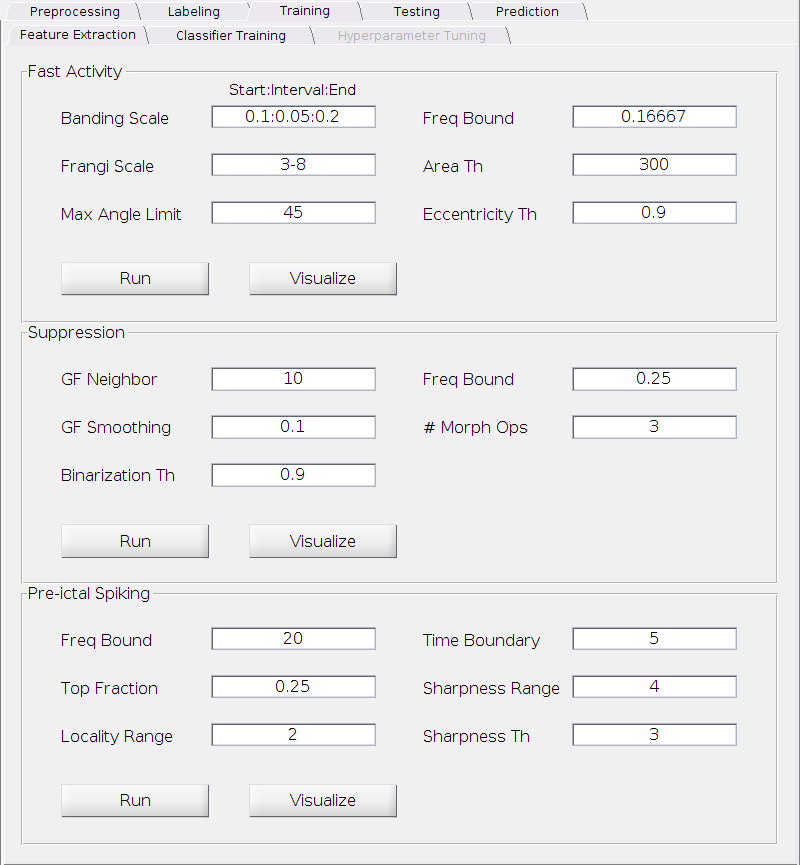
The features will be extracted for fast activity, suppression and pre-ictal spikes in this section. Once you set the parameters, click Run in each of three sub-panel to extract the corresponding features. Note the suppression extraction depends on the results of the fast activity. i.e. if you re-run the fast activity panel, you have to re-run suppression panel as well.
Fast Activity
Banding Scale:
The multiple scales for the detection of fast activity with different intensities. Lower end reflects the detection ability for strong (relative bright) bandings and the higher end reflects the detection ability for weak (relative dark) bandings. The input format is x:y:z, where x is the starting scale, y is the interval and z is the ending scale (It’s a standard MATLAB notation). For example, 0.1:0.1:0.3 represents 3 scales (0.1, 0.2, 0.3) in total.
Requirement: All positive real numbers between 0 and 0.5; x <= zand y <= z.
Default: 0.1:0.05:0.2.
Frangi Scale:
We use Frangi filter[3] to detect banding structures with different widths. This is the spatial scale for the Frangi filter. The input format is x-y, where x is the starting scale and y is the ending scale. Both x and y are positive integers.
Requirement: All positive integers; x < y.
Default: 3-8.
Max Angle Limit:
The threshold on the (absolute) angle of bandings in degree to remove false positive detection. Anything beyond this value or below the negative of this value will be discarded.
Requirement: A positive real number between 0 and 90.
Default: 45.
Freq Bound:
The threshold on the position of the bandings relative to the frequency boundaries (top and bottom edges of the TF plot) to remove false positive detection. Anything near the either of the boundaries within a certain range (this value x total number of frequency bins) will be discarded. For example, suppose we set frequency range to be 1:1:200 when computing the TF plot (therefore 200 frequency bins in total) and we set this threshold to be 0.1. Then any banding below 20 Hz or beyond 180 will not be detected.
Requirement: A positive real number between 0 and 0.5.
Default: 1/6
Area Th:
The threshold on the size of the detected banding area to remove false positive detection in pixel. Anything below this value will be discarded.
Requirement: A positive real number.
Default: 300.
Eccentricity Th:
The threshold on the eccentricity of the detected banding area to remove false positive detection in pixel. Anything below this value will be discarded.
Requirement: A positive real number between 0 and 1.
Default: 0.9.
A tick in the “FA” column will show up in the Data panel for each of the seizures of your selection, indicating the completion of this step.
Suppression
GF Neighbor:
The edge-preserving Guided filter[3] is applied to smooth the TF plot in the first step of suppression detection. This parameter is the neighborbood size of the Guided filter.
Requirement: A positive integer.
Default: 10.
GF Smoothing:
Similar to the one above, this parameter is the degree of smoothing of the Guided filter.
Requirement: A positive real number.
Default: 0.1.
Binarization Th:
The threshold for binarization of the smoothed image. The higher, the smaller the detected suppression region.
Requirement: A positive real number between 0 and 1.
Default: 0.9.
Freq Bound:
The upper bound for the suppression detection. Anything above this bound will be discarded. See the “Freq Bound” of the fast activity for how to interpret this number.
Requirement: A positive real number between 0 and 1.
Default: 0.25.
# Morph Ops:
The number of morphological operations (see MATLAB open and close functions) performed to clean up the result.
Requirement: A positive integer.
Default: 3.
A tick in the “SP” column will show up in the Data panel for each of the seizures of your selection, indicating the completion of this step.
Pre-ictal Spikes
Freq Bound:
The lower frequency bound for the spike detection to remove the blurring effect of the wavelet computation. Anything below this bound will be discarded before further steps. See the “Freq Bound” of the fast activity for how to interpret this number.
Requirement: A positive real number between 0 and 1.
Default: 0.1.
Top Fraction:
The frequency response at each time point will be sorted in a descending order and only the top portion will be used for characterize the strength of the response. This parameter control the fraction level.
Requirement: A positive real number between 0 and 1.
Default: 0.25.
Time Boundary:
The detection of spikes near the either the beginning or the end of the pre-ictal period is usually not accurate. Hence we remove possible false detections if it’s within this many of time points near either boundaries.
Requirement: A positive integer.
Default: 5.
Sharpness Range:
The neighborbood size (number of time points) used to characterize the sharpness of the spikes.
Requirement: A positive integer.
Default: 4.
Sharpness Th:
The threshold of the ratio between the sharpness of the spike and the counterpart of its neighbors. Any spike with ratio below this threshold will be removed from candidacy.
Requirement: A positive real number.
Default: 3.
A tick in the “PS” column will show up in the Data panel for each of the seizures of your selection, indicating the completion of this step.
Visualization of the Extracted Features
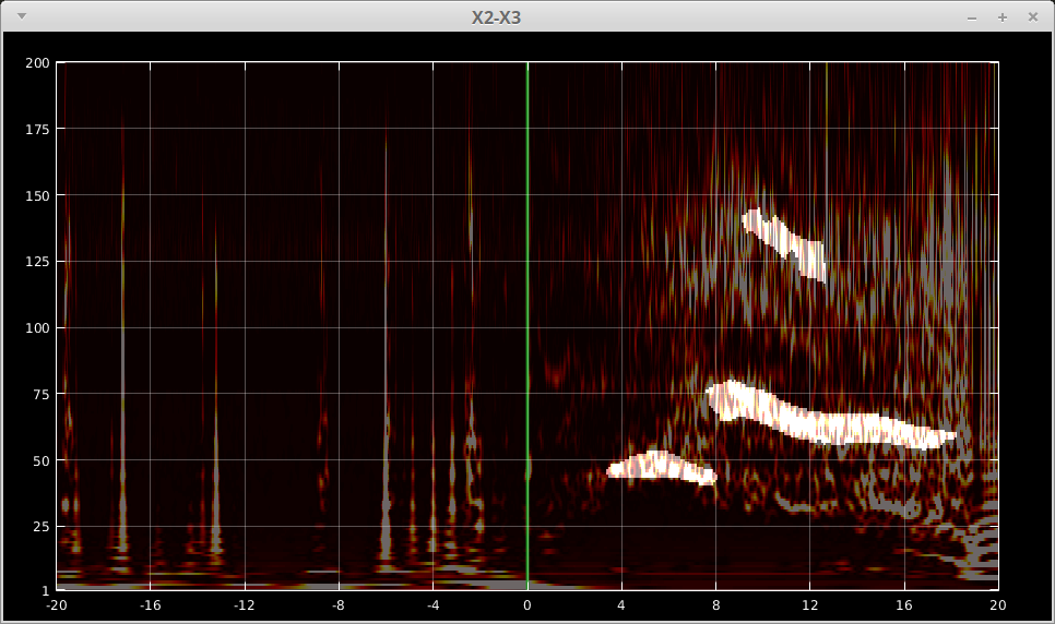
In each of the three sub-panels, we provide a way to visualize the extracted features. Click Visualize button to open the TF plots with semi-transparent masks of the extracted feature. Then you may click a single TF plot to check the result for a particular contact. An example of fast acitivty feature is shown below.
You may press:
m- to toggle the mask on and off.,- to increase the transparency (less mask, more image)..- to decrease the transparency (more mask, less image).
Classifier Training
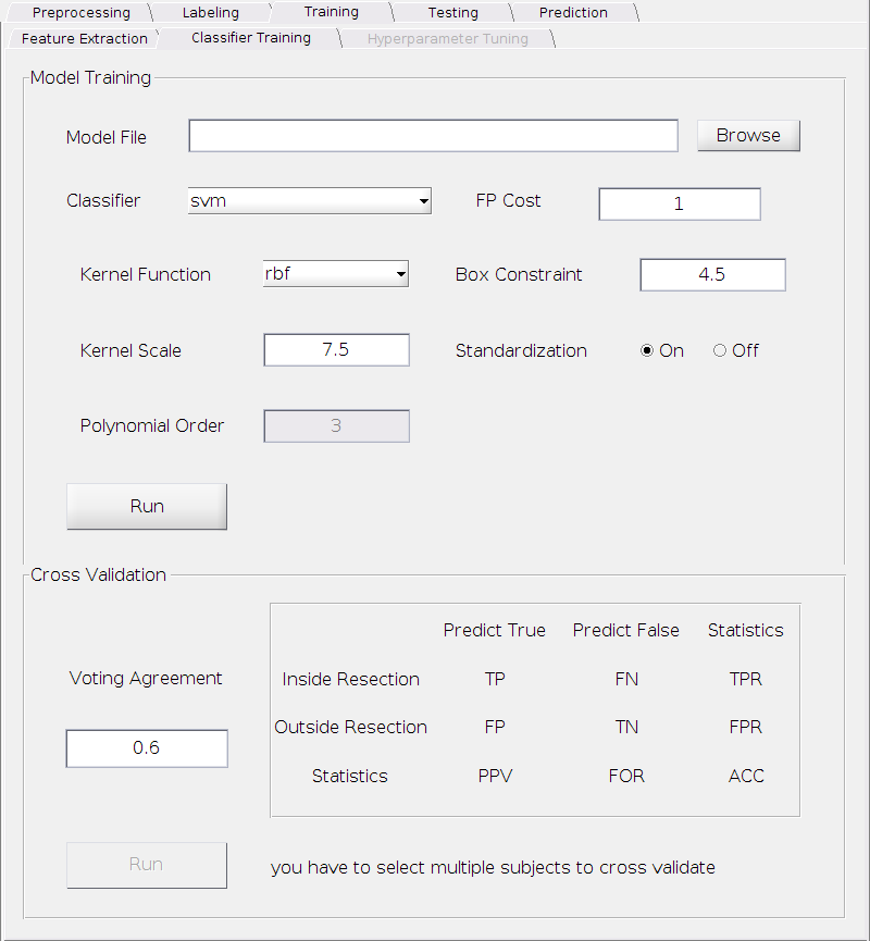
With the features we extracted above and the labels marked for the resected region, we can now train a classifier. The figure below shows the classifier training panel.
Model Training
With the top sub-panel “Model Training”, you can select a classifier, set its parameters, train a model and save it into disk. Currently we only implemented the SVM classifier as described in the paper. For a SVM classifier, you can tune the following parameters. Since we used the MATLAB built-in SVM function, for the meaning of each parameter, see MATLAB SVM explanation and fitcsvm
Kernel Function:
Requirement: Select one among the drop down menu: linear, rbf (Gaussian) and polynomial.
Default: rbf.
Kernel Scale:
Requirement: A positive real number.
Default: 7.5.
Polynomial Order:
Requirement: Only valid when the kernel function is set to polynomial and it’s a positive integer, typically among 2, 3 or 4, rarely go beyond 5.
Default: 3.
FP Cost:
The penalty weight applied to false positive. A false positive contact is defined as the one that is outside the resected area but predicted as EZ contacts by the classifier. See the “Cost” parameter of the fitcsvm function.
Requirement: A positive real number.
Default: 1.
Standarization:
Requirement: Choose either on or off.
Default: off
Once you fixed the parameters, click the Browse button to locate a place to save your model to disk. Simply enter a new file name without an extension to save a new model or you can confirm and overwrite an old one if you want. A model will be save to your desired place with an extension “.model”. We make this extension on purpose to avoid potential confusion with other files.
Finally, don’t forget to click Run button to actually train and save the model.
Cross-validation
Although you can set the parameters and train a classification model now, how would you know if this model will perform well or not when predicting EZ for a new subject? In fact, the performance of the classifier may be sensitive to the choice of the parameters for some given dataset. Therefore a cross-validation is highly desired to make sure the choice of the parameters are proper to yield a reasonable prediction result (i.e. to avoid overfitting problem). The bottom sub-panel provides a way for cross-validations.
Before cross-validation, you need to:
Select multiple subjects (more than one).
This is required by our subject-based cross-validation strategy.
Set the “Voting Agreement”.
Usually, we may have multiple seizures for a particular subject. The more seizure data we collected, the more reliable we can predict the EZ as if the majority of the seizures agree with each other that the fingerprint appears on a particular contacts, then it’s very likely that this is a EZ contact.
Hence, the “Voting Agreement” here is the threshold of the fraction of seizures that need to agree with each other in order to predict as EZ for a particular contact.
Requirement: A positive real number between 0 and 1.
Default: 0.6.
Now you can click Run button to perform the cross-validation. The result will appear on the right side of this panel. The top left 2 x 2 sub-matrix shows how many contacts within/outside the resection that are predicted true/false(EZ/non-EZ contact). And the third row and the third column shows some standard statistics for a binary confusion matrix.
You may play with different parameters on the top and run the cross-validation to check the performance. Once you are satisfied with your parameter settings, you can use that set of parameter to train a model and save to disk for later testing and/or prediction usage.
Hyperparameter Tuning (Experimental)
Sometimes it’s a little tedious to try different combinations of the parameters to acheive the best cross-validation result. Hence, we provide an extra functionality to help you tune the parameters automatically. However, this feature is experimental and is not always guaranteed to find you the best parameters, depending your dataset, the searching ranges for different parameters, how long will you run it and etc. (Technically speaking, it’s not guaranteed because the optimization of the hyperparameters is a highly non-convex problem).
Although it’s not mature yet, we encourage you:
Give a try and be careful and always double check the returned parameters to see if they are reasonable to you.
For advanced users, use the our MATLAB function as a template and customize it based on your need.
The hyperparameter tuning procedure fully depends on the Bayesian optimization algorithm provided by MATLAB.
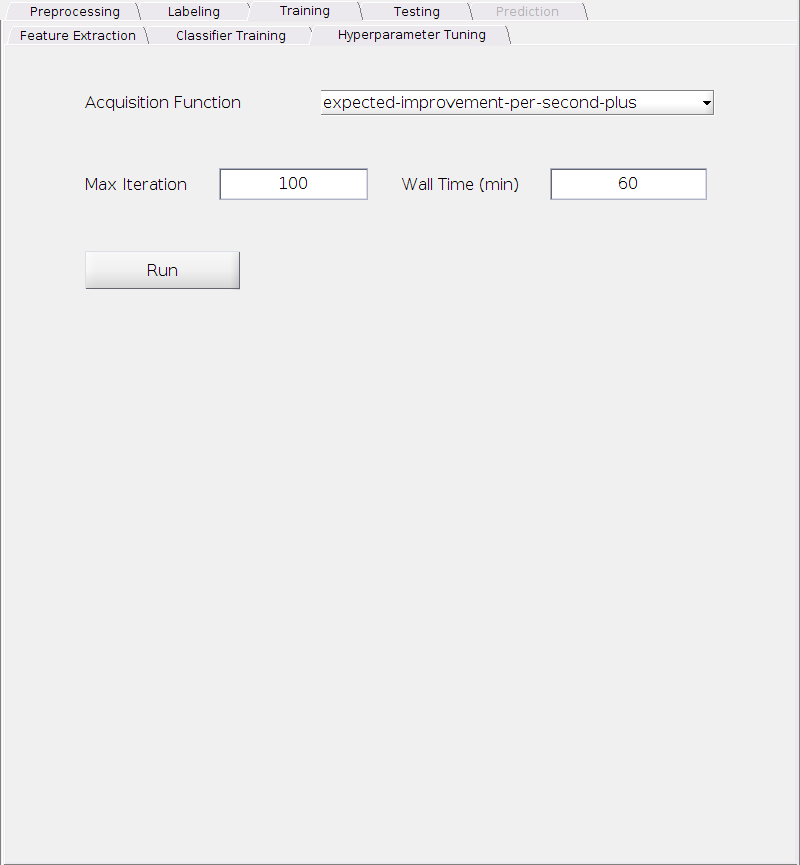
Acquisition Function:
Requirement: Choose one from the following:
- expected-improvement-per-second-plus
- expected-improvement
- expected-improvement-plus
- expected-improvement-per-second
- lower-confidence-bound
- probability-of-improvement
- grid
- random
Default: expected-improvement-per-second-plus
Max Iteration:
Requirement: A positive integer.
Default: 100.
Wall Time (min):
Requirement: A positive integer.
Default: 60.
After set all paramters, hit Run button to start tuning. A report will be dynamically updated and displayed at the bottom of this tab to show the progress. An example of the progress is shown below:
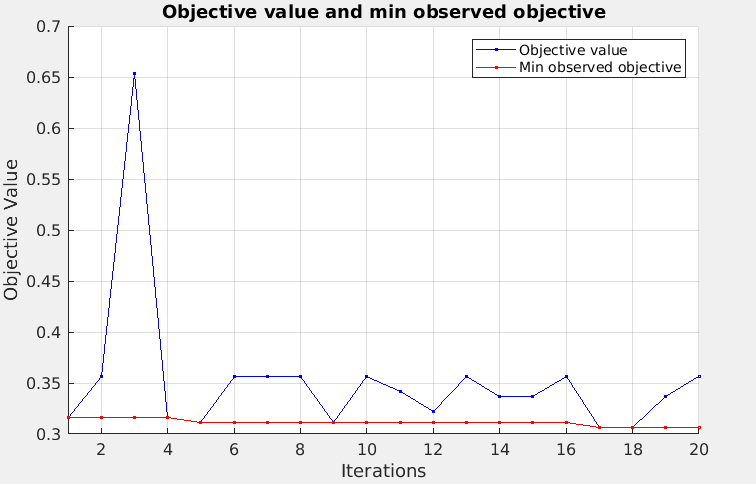
Also numberical results at each search step will be shown in the MATLAB command window. The tunning process will be terminated if either the maximum number of iterations exceeds the specified limit or the running time exceeds the wall time. The final results (best parameters found during the searching) will be displayed then. Right-click the bottom panel will toggle to the progress report and Left-click that will toggle back to the results.
Reference
[1] Support-vector networks, Machine Learning, vol. 20, no. 3, pp. 273-297, 1995.
[2] A fingerprint of the epileptogenic zone in human epilepsies, Brain, vol. 141, no. 1, pp. 117-131, 2017.
[3] Multiscale vessel enhancement filtering, International Conference on Medical Image Computing and Computer-Assisted Intervention, pp. 130-137. Springer, Berlin, Heidelberg, 1998.
[4] Guided image filtering, IEEE transactions on pattern analysis and machine intelligence, vol. 35, no. 6, pp. 1397-1409, 2013.